初识 TensorFlow

本指南让你开始进行 TensorFlow 编程。开始之前，安装 TensorFlow， 为了充分利用本指南，您应该了解以下内容：

• Python 如何编程。
• 至少对数组了解一点。
• 最好了解一些机器学习。然而，如果你对机器学习了解很少或不了解，你仍然应该首先阅读本指南。

TensorFlow 提供了多种API。最底层的 API--TensorFlow Core-- 可以让你完全控制自己的程序。 我们推荐机器学习研究人员和其他需要很好控制他们的模型的人员使用TensorFlow Core。 更高级别的API构建在 TensorFlow Core 之上。这些更高级的API通常比 TensorFlow Core 更容易学习和使用。此外，较高级别的 API 使重复任务更容易，不同用户之间更一致。像 tf.contrib.learn 这样的高级API可以帮助您管理数据集，进行估计，训练和推理。注意：一些高级 API（名称包含contrib的API）仍然在开发中。 有些contrib方法之后可能会改变或在随后的 TensorFlow 版本中废弃。

本指南从 TensorFlow Core 的教程开始。随后我们会演示如何通过 tf.contrib.learn 实现相同的模型。 了解 TensorFlow Core 的原理将你您提供一个 mental model，以便你在使用更紧凑更高级的 API 时理解内部是如何工作的

Tensors

The central unit of data in TensorFlow is the tensor. A tensor consists of a set of primitive values shaped into an array of any number of dimensions. A tensor's rank is its number of dimensions. Here are some examples of tensors:

3 # a rank 0 tensor; this is a scalar with shape []
[1. ,2., 3.] # a rank 1 tensor; this is a vector with shape [3]
[[1., 2., 3.], [4., 5., 6.]] # a rank 2 tensor; a matrix with shape [2, 3]
[[[1., 2., 3.]], [[7., 8., 9.]]] # a rank 3 tensor with shape [2, 1, 3]

TensorFlow Core tutorial

Importing TensorFlow

The canonical import statement for TensorFlow programs is as follows:

import tensorflow as tf

This gives Python access to all of TensorFlow's classes, methods, and symbols. Most of the documentation assumes you have already done this.

The Computational Graph

You might think of TensorFlow Core programs as consisting of two discrete sections:

1. Building the computational graph.
2. Running the computational graph.

A computational graph is a series of TensorFlow operations arranged into a graph of nodes. Let's build a simple computational graph. Each node takes zero or more tensors as inputs and produces a tensor as an output. One type of node is a constant. Like all TensorFlow constants, it takes no inputs, and it outputs a value it stores internally. We can create two floating point Tensors node1 and node2 as follows:

node1 = tf.constant(3.0, tf.float32)
node2 = tf.constant(4.0) # also tf.float32 implicitly
print(node1, node2)

The final print statement produces

Tensor("Const:0", shape=(), dtype=float32) Tensor("Const_1:0", shape=(), dtype=float32)

Notice that printing the nodes does not output the values 3.0 and 4.0 as you might expect. Instead, they are nodes that, when evaluated, would produce 3.0 and 4.0, respectively. To actually evaluate the nodes, we must run the computational graph within a session. A session encapsulates the control and state of the TensorFlow runtime.

The following code creates a Session object and then invokes its run method to run enough of the computational graph to evaluate node1 and node2. By running the computational graph in a session as follows:

sess = tf.Session()
print(sess.run([node1, node2]))

we see the expected values of 3.0 and 4.0:

[3.0, 4.0]

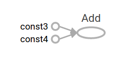
We can build more complicated computations by combining Tensor nodes with operations (Operations are also nodes.). For example, we can add our two constant nodes and produce a new graph as follows:

node3 = tf.add(node1, node2)
print("node3: ", node3)
print("sess.run(node3): ",sess.run(node3))

The last two print statements produce

node3:  Tensor("Add_2:0", shape=(), dtype=float32)
sess.run(node3):  7.0

TensorFlow provides a utility called TensorBoard that can display a picture of the computational graph. Here is a screenshot showing how TensorBoard visualizes the graph:

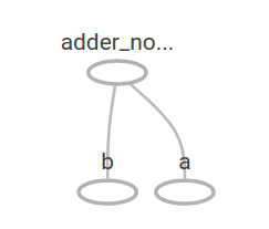
As it stands, this graph is not especially interesting because it always produces a constant result. A graph can be parameterized to accept external inputs, known as placeholders. A placeholder is a promise to provide a value later.

a = tf.placeholder(tf.float32)
b = tf.placeholder(tf.float32)
adder_node = a + b  # + provides a shortcut for tf.add(a, b)

The preceding three lines are a bit like a function or a lambda in which we define two input parameters (a and b) and then an operation on them. We can evaluate this graph with multiple inputs by using the feed_dict parameter to specify Tensors that provide concrete values to these placeholders:

print(sess.run(adder_node, {a: 3, b:4.5}))
print(sess.run(adder_node, {a: [1,3], b: [2, 4]}))

resulting in the output

7.5
[ 3.  7.]

In TensorBoard, the graph looks like this:

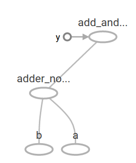
We can make the computational graph more complex by adding another operation. For example,

add_and_triple = adder_node * 3.
print(sess.run(add_and_triple, {a: 3, b:4.5}))

produces the output

22.5

The preceding computational graph would look as follows in TensorBoard:

In machine learning we will typically want a model that can take arbitrary inputs, such as the one above. To make the model trainable, we need to be able to modify the graph to get new outputs with the same input. Variables allow us to add trainable parameters to a graph. They are constructed with a type and initial value:

W = tf.Variable([.3], tf.float32)
b = tf.Variable([-.3], tf.float32)
x = tf.placeholder(tf.float32)
linear_model = W * x + b

Constants are initialized when you call tf.constant, and their value can never change. By contrast, variables are not initialized when you call tf.Variable. To initialize all the variables in a TensorFlow program, you must explicitly call a special operation as follows:

init = tf.global_variables_initializer()
sess.run(init)

It is important to realize init is a handle to the TensorFlow sub-graph that initializes all the global variables. Until we call sess.run, the variables are uninitialized.

Since x is a placeholder, we can evaluate linear_model for several values of x simultaneously as follows:

print(sess.run(linear_model, {x:[1,2,3,4]}))

to produce the output

[ 0.          0.30000001  0.60000002  0.90000004]

We've created a model, but we don't know how good it is yet. To evaluate the model on training data, we need a y placeholder to provide the desired values, and we need to write a loss function.

A loss function measures how far apart the current model is from the provided data. We'll use a standard loss model for linear regression, which sums the squares of the deltas between the current model and the provided data. linear_model - y creates a vector where each element is the corresponding example's error delta. We call tf.square to square that error. Then, we sum all the squared errors to create a single scalar that abstracts the error of all examples using tf.reduce_sum:

y = tf.placeholder(tf.float32)
squared_deltas = tf.square(linear_model - y)
loss = tf.reduce_sum(squared_deltas)
print(sess.run(loss, {x:[1,2,3,4], y:[0,-1,-2,-3]}))

producing the loss value

23.66

We could improve this manually by reassigning the values of W and b to the perfect values of -1 and 1. A variable is initialized to the value provided to tf.Variable but can be changed using operations like tf.assign. For example, W=-1 and b=1 are the optimal parameters for our model. We can change W and b accordingly:

fixW = tf.assign(W, [-1.])
fixb = tf.assign(b, [1.])
sess.run([fixW, fixb])
print(sess.run(loss, {x:[1,2,3,4], y:[0,-1,-2,-3]}))

The final print shows the loss now is zero.

0.0

We guessed the "perfect" values of W and b, but the whole point of machine learning is to find the correct model parameters automatically. We will show how to accomplish this in the next section.

tf.train API

A complete discussion of machine learning is out of the scope of this tutorial. However, TensorFlow provides optimizers that slowly change each variable in order to minimize the loss function. The simplest optimizer is gradient descent. It modifies each variable according to the magnitude of the derivative of loss with respect to that variable. In general, computing symbolic derivatives manually is tedious and error-prone. Consequently, TensorFlow can automatically produce derivatives given only a description of the model using the function tf.gradients. For simplicity, optimizers typically do this for you. For example,

optimizer = tf.train.GradientDescentOptimizer(0.01)
train = optimizer.minimize(loss)

sess.run(init) # reset values to incorrect defaults.
for i in range(1000):
  sess.run(train, {x:[1,2,3,4], y:[0,-1,-2,-3]})

print(sess.run([W, b]))

results in the final model parameters:

[array([-0.9999969], dtype=float32), array([ 0.99999082],
 dtype=float32)]

Now we have done actual machine learning! Although doing this simple linear regression doesn't require much TensorFlow core code, more complicated models and methods to feed data into your model necessitate more code. Thus TensorFlow provides higher level abstractions for common patterns, structures, and functionality. We will learn how to use some of these abstractions in the next section.

Complete program

The completed trainable linear regression model is shown here:

import numpy as np
import tensorflow as tf

# Model parameters
W = tf.Variable([.3], tf.float32)
b = tf.Variable([-.3], tf.float32)
# Model input and output
x = tf.placeholder(tf.float32)
linear_model = W * x + b
y = tf.placeholder(tf.float32)
# loss
loss = tf.reduce_sum(tf.square(linear_model - y)) # sum of the squares
# optimizer
optimizer = tf.train.GradientDescentOptimizer(0.01)
train = optimizer.minimize(loss)
# training data
x_train = [1,2,3,4]
y_train = [0,-1,-2,-3]
# training loop
init = tf.global_variables_initializer()
sess = tf.Session()
sess.run(init) # reset values to wrong
for i in range(1000):
  sess.run(train, {x:x_train, y:y_train})

# evaluate training accuracy
curr_W, curr_b, curr_loss  = sess.run([W, b, loss], {x:x_train, y:y_train})
print("W: %s b: %s loss: %s"%(curr_W, curr_b, curr_loss))

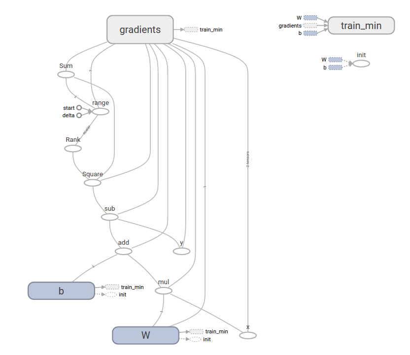
When run, it produces

W: [-0.9999969] b: [ 0.99999082] loss: 5.69997e-11

This more complicated program can still be visualized in TensorBoard

tf.contrib.learn

tf.contrib.learn is a high-level TensorFlow library that simplifies the mechanics of machine learning, including the following:

• running training loops
• running evaluation loops
• managing data sets
• managing feeding

tf.contrib.learn defines many common models.

Basic usage

Notice how much simpler the linear regression program becomes with tf.contrib.learn:

import tensorflow as tf
# NumPy is often used to load, manipulate and preprocess data.
import numpy as np

# Declare list of features. We only have one real-valued feature. There are many
# other types of columns that are more complicated and useful.
features = [tf.contrib.layers.real_valued_column("x", dimension=1)]

# An estimator is the front end to invoke training (fitting) and evaluation
# (inference). There are many predefined types like linear regression,
# logistic regression, linear classification, logistic classification, and
# many neural network classifiers and regressors. The following code
# provides an estimator that does linear regression.
estimator = tf.contrib.learn.LinearRegressor(feature_columns=features)

# TensorFlow provides many helper methods to read and set up data sets.
# Here we use `numpy_input_fn`. We have to tell the function how many batches
# of data (num_epochs) we want and how big each batch should be.
x = np.array([1., 2., 3., 4.])
y = np.array([0., -1., -2., -3.])
input_fn = tf.contrib.learn.io.numpy_input_fn({"x":x}, y, batch_size=4,
                                              num_epochs=1000)

# We can invoke 1000 training steps by invoking the `fit` method and passing the
# training data set.
estimator.fit(input_fn=input_fn, steps=1000)

# Here we evaluate how well our model did. In a real example, we would want
# to use a separate validation and testing data set to avoid overfitting.
print(estimator.evaluate(input_fn=input_fn))

When run, it produces

    {'global_step': 1000, 'loss': 1.9650059e-11}

A custom model

tf.contrib.learn does not lock you into its predefined models. Suppose we wanted to create a custom model that is not built into TensorFlow. We can still retain the high level abstraction of data set, feeding, training, etc. of tf.contrib.learn. For illustration, we will show how to implement our own equivalent model to LinearRegressor using our knowledge of the lower level TensorFlow API.

To define a custom model that works with tf.contrib.learn, we need to use tf.contrib.learn.Estimator. tf.contrib.learn.LinearRegressor is actually a sub-class of tf.contrib.learn.Estimator. Instead of sub-classing Estimator, we simply provide Estimator a function model_fn that tells tf.contrib.learn how it can evaluate predictions, training steps, and loss. The code is as follows:

import numpy as np
import tensorflow as tf
# Declare list of features, we only have one real-valued feature
def model(features, labels, mode):
  # Build a linear model and predict values
  W = tf.get_variable("W", [1], dtype=tf.float64)
  b = tf.get_variable("b", [1], dtype=tf.float64)
  y = W*features['x'] + b
  # Loss sub-graph
  loss = tf.reduce_sum(tf.square(y - labels))
  # Training sub-graph
  global_step = tf.train.get_global_step()
  optimizer = tf.train.GradientDescentOptimizer(0.01)
  train = tf.group(optimizer.minimize(loss),
                   tf.assign_add(global_step, 1))
  # ModelFnOps connects subgraphs we built to the
  # appropriate functionality.
  return tf.contrib.learn.ModelFnOps(
      mode=mode, predictions=y,
      loss=loss,
      train_op=train)

estimator = tf.contrib.learn.Estimator(model_fn=model)
# define our data set
x = np.array([1., 2., 3., 4.])
y = np.array([0., -1., -2., -3.])
input_fn = tf.contrib.learn.io.numpy_input_fn({"x": x}, y, 4, num_epochs=1000)

# train
estimator.fit(input_fn=input_fn, steps=1000)
# evaluate our model
print(estimator.evaluate(input_fn=input_fn, steps=10))

When run, it produces

{'loss': 5.9819476e-11, 'global_step': 1000}

Notice how the contents of the custom model() function are very similar to our manual model training loop from the lower level API.

Next steps

Now you have a working knowledge of the basics of TensorFlow. We have several more tutorials that you can look at to learn more. If you are a beginner in machine learning see @{$beginners$MNIST for beginners}, otherwise see @{$pros$Deep MNIST for experts}.